Create a Retrieval#
This section describes how to create a retrieval using the openMWR package.
The main steps are:
Create the site configuration
Download and prepare the training data
Run the forward calculation
Separate in training, validation, and test datasets
Create an analysis dataset from real measurements
Train the retrieval model
All the code snippets below can be found in the python script bin/main.py.
It is recommended to run the script step by step and comment out the parts that are not needed.
The script can be run from the command line as follows:
cd bin/
./run_py_script.sh main.py
run_py_script.sh runs the script automatically with the activated venv environment (created in Installation).
It uses the nohup command to keep it running after closing the terminal.
The logging output is saved in bin/main.py.log.
All the data generated below is saved in the path set in the variable DATA_DIR.
DATA_DIR = '../data'
Create the Site Configuration#
Before you can create a retrieval, you need to set up the site configuration. This includes defining the site name, location, and any other relevant parameters for a specific microwave radiometer. Here is an example of how to create a site configuration for the G5 Hatpro in munich:
from openMWR.site import create_site

site = 'munich_G5'
create_site(
            site,
            data_dir=DATA_DIR,
            hatpro_data_dir="/project/meteo/data/hatpro-g5",
            retrieval_output_dir="/project/meteo/data/hatpro-g5/mim_retrieval",
            gen='G5',
            mwr_height=550,
            rpg_retrieval_exists = True,
            mwr_measurement_start_date = '2024-11-01',
            latitude = 48.148,
            longitude = 11.573,
            plot_dir='/project/meteo/homepages/quicklooks/hatpro/G5'
            )
(See openMWR.site.create_site())
hatpro_data_dir is the directory where the MWR data is stored.
It should contain subfolders for each year, e.g. ‘Y2025’, ‘Y2024’, etc.
gen is the generation of the Hatpro MWR (G4 or G5).
mwr_height is the height of the MWR above sea level in meters.
rpg_retrieval_exists indicates whether an RPG retrieval is available for the site.
mwr_measurement_start_date is the date when the MWR measurements start (format: ‘YYYY-MM-DD’).
latitude and longitude are the coordinates of the site.
plot_dir (optional) is the directory where the plots will be saved, when it is run optionally with e.g. bin/cron_job.py (see Run Operational).
retrieval_output_dir (optional) is the directory where the retrieval results will be saved, when it is run optionally with e.g. bin/cron_job.py (see Run Operational).
The function create_site creates a folder in {DATA_DIR}/sites/ with the site name and saves the site configuration in a JSON file in that folder.
Download and Prepare the Training Data#
To generate training data, either the measurement data from radiosondes or era5 data can be used. The recommended option is to use radiosonde data, as it provides more accurate and higher-resolution profiles of atmospheric parameters. It has also been tested more extensively.
Radiosonde Data#
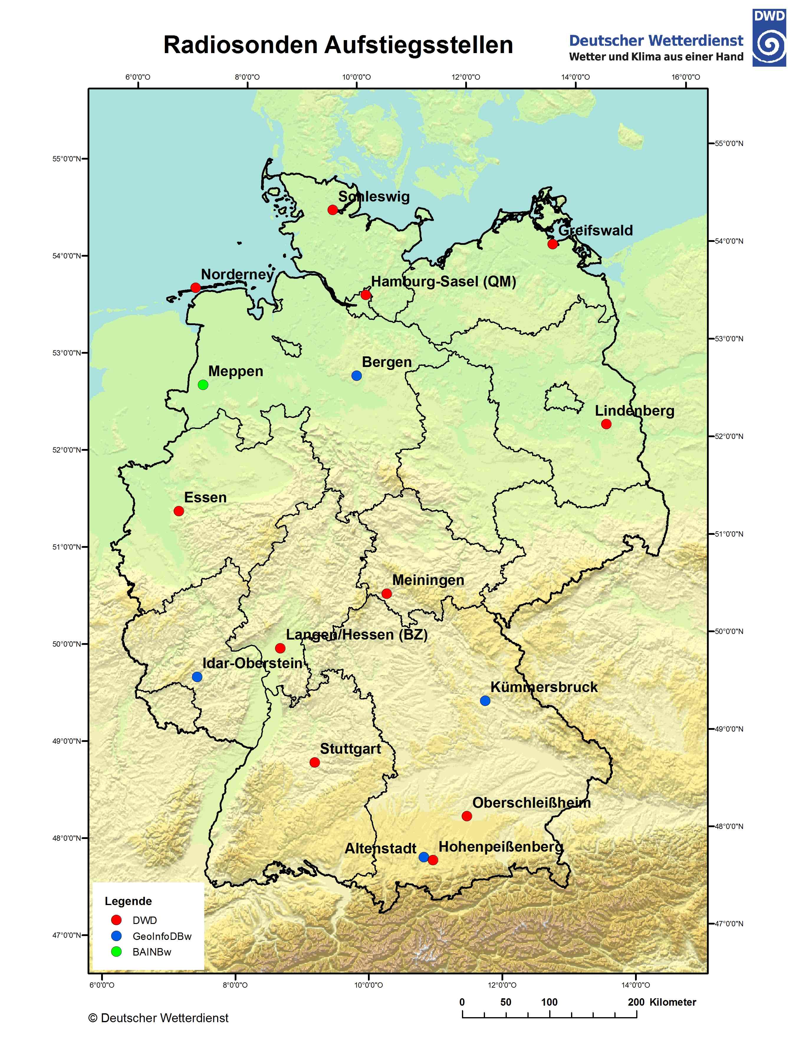
The first step is deciding which radiosonde stations to use for the training data. Currently, only radiosondes from the German weather service can be downloaded. For sites outside of Germany, a download option must first be implemented. Below is a map of radiosonde stations in Germany, along with a table of their station IDs. It is useful to use the stations that are closest to the MWR site. For the example of Munich, the Oberschleißheim station alone was enough as it had data since 1990 and about 20000 usable profiles.
Station Id |
Name |
Height (m) |
Latitude |
Longitude |
|---|---|---|---|---|
00125 |
Altenstadt |
760 |
47.8342 |
10.8667 |
00368 |
Bergen |
69 |
52.8152 |
9.9248 |
01303 |
Essen-Bredeney |
150 |
51.4041 |
6.9677 |
01757 |
Greifswald |
2 |
54.0967 |
13.4056 |
02290 |
Hohenpeißenberg |
977 |
47.8009 |
11.0108 |
02385 |
Idar-Oberstein |
376 |
49.6927 |
7.3263 |
02773 |
Kümmersbruck |
416 |
49.4283 |
11.9016 |
03015 |
Lindenberg |
98 |
52.2085 |
14.118 |
03231 |
Meiningen |
450 |
50.5611 |
10.3771 |
03254 |
Meppen |
19 |
52.7155 |
7.3176 |
03631 |
Norderney |
12 |
53.7123 |
7.1519 |
03715 |
Oberschleißheim (Lustheim) |
484 |
48.2446 |
11.5525 |
04466 |
Schleswig |
43 |
54.5275 |
9.5487 |
04928 |
Stuttgart (Schnarrenberg) |
314 |
48.8281 |
9.2 |
06202 |
Oppin |
106 |
51.5467 |
12.0608 |
Source: DWD
The download process is separated into two steps. First, the raw radiosonde data is downloaded and saved locally. Then, the data is processed and prepared for radiative transfer calculations. This first step is independent of any site configuration, and the data can be reused for multiple sites. The only thing that needs to be specified is the start and end years between which the program will try to download the data. The default end year is the current year.
from openMWR.dwd_opendata import download_radiosondes

station_ids = ['03715'] # Oberschleißheim
for station_id in station_ids:
    download_radiosondes(station_id, data_dir=DATA_DIR, start_year=1990)
(See openMWR.dwd_opendata.download_radiosondes())
The second step involves processing and preparing the downloaded raw data for the radiative transfer calculation. Among more filtering steps, the function does the following:
Loads the raw radiosonde data files for the specified station.
Filters out all profiles that do not reach a height of 15 km.
Adds a liquid water content (LWC) profile calculated using the adiabatic model. (See
openMWR.cloud)Changes the height coordinate to height above ground level.
Interpolates the profiles to a specified set of heights.
Fills in missing values caused by the radiosonde not reaching the maximum height using the monthly mean of the available profiles.
Adds derived data, such as absolute humidity, dew point, LWP and IWV.
In order to run the function, one must provide a height grid in form of a numpy array for interpolation. This grid will also be the output grid for the retrieval. (Note that the output grid can be a subset of the original grid.)
The standard heights used in openMWR can be imported from openMWR.consts.
For the zero height, either the radiosonde station height or the MWR height can be used. In the latter case, the radiosonde profiles are cut off. This is recommended when the MWR height is significantly higher than the radiosonde station height. This behavior can be configured using the parameter cut_off_at_mwr_height.
from openMWR.radiosonde import create_radiosonde_dataset_for_RT
from openMWR.consts import std_heights

for station_id in station_ids:
    create_radiosonde_dataset_for_RT(
        site,
        station_id,
        data_dir=DATA_DIR,
        heights=std_heights,
        cut_off_at_mwr_height=False,
    )
Era5 Data#
The era5 data can be used as an alternative to radiosonde data for training data generation but also for analysis of the retrieval.
The era5 data is downloaded and processed using the ERA5Processor class. After creating an instance of the class with the site name, the raw data dataset can be created using the create_original_dataset method. The method has an option to set the temporal frequency of the data (in hours). The default is 6 hour. A start and end date can also be specified. The default values are the mwr_measurement_start_date from the site configuration until 5 days before the current date.
from openMWR.era5 import ERA5Processor

era5 = ERA5Processor(site, data_dir=DATA_DIR, start_date='2025-01-01')
era5.create_original_dataset(h_freq=2)
(See openMWR.era5.ERA5Processor and openMWR.era5.ERA5Processor.create_original_dataset())
Run the forward calculation#
The forward calculation for the radiosonde data can be run using the create_radiosonde_dataset_with_RT function from openMWR.radiosonde. Internally this calls openMWR.run_RT.run_RT() and supports two microwave RT backends: TorchMWRT (default) and pyrtlib. For the infrared sensor on the MWR, libradtran is used.
The arguments of the function are the station ID, the site name, the data directory, and the frequencies and elevation angles for which the brightness temperatures should be calculated. The angles only need to be specified if boundary layer scans with the MWR are performed and a retrieval for these is planned. The default angles are set to 90 degrees only. For the frequencies and angles standard values can be imported from openMWR.consts.
There is also an option to use a frequency shift for each channel, which will be subtracted from the original frequencies for the calculation. To use a frequency shift, use the argument freq_shift and provide a numpy array with the same length as the frequencies array.
It is recommended to use multiprocessing to speed up the calculation. The number of processes can be set using the num_of_processes argument. All the radiosonde profiles will be distributed to the processes equally and then calculated in parallel. The maximum number of processes should not exceed the number of CPU cores available on the machine. To get the maximum number of CPU cores available, os.cpu_count() can be used.
If TorchMWRT is used as RT backend, multiprocessing is not used for the forward calculation of the brightness temperatures, because it is not nessecary. I usually just takes a few minuits, because it is havily vectorized. The num_of_processes argument is then only used for the forward calculation of the infrared brightness temperature with libradtran.
from openMWR.radiosonde import create_radiosonde_dataset_with_RT
from openMWR.consts import std_freqs, std_angles

for station_id in station_ids:
    create_radiosonde_dataset_with_RT(
        station_id,
        site,
        data_dir=DATA_DIR,
        freqs=std_freqs,
        angles=std_angles,
        num_of_processes=20,
        RT_model='torchMWRT',
    )
(See openMWR.radiosonde.create_radiosonde_dataset_with_RT())
The forward calculation for the ERA5 data can be run using the create_forward_calc_dataset method of the ERA5Processor class. The arguments are similar to those of the create_radiosonde_dataset_with_RT function, including the optional RT_model argument. The number of processes can also be set to speed up the calculation. In case of the era5 data, the interpolation to the specified heights is also performed during the forward calculation.
era5.create_forward_calc_dataset(std_freqs, std_heights, std_angles, num_of_processes=12)
(See openMWR.era5.ERA5Processor.create_forward_calc_dataset())
Separate in training, validation, and test datasets#
The forward calculation datasets that were created need to be separated into training, validation, and test datasets. This can be done using the separate_training_data function from the openMWR.train module. The source argument needs to be set to either a radiosonde station ID (for example '03715') or 'era5'. The function randomly selects 10% of the time indices for the test dataset and another 10% for the validation dataset. The remaining 80% of the data is used for training. These fractions can be adjusted using the test_fraction and val_fraction arguments.
from openMWR.train import separate_training_data

for station_id in station_ids:
    separate_training_data(site, source=station_id, data_dir=DATA_DIR)
or
separate_training_data(site, source='era5', data_dir=DATA_DIR)
Create an analysis dataset from real measurements#
An analysis dataset is a collection of real measurements with corresponding atmospheric profiles. It is not strictly necessary for training the retrieval model, but it is useful to evaluate the performance of the retrieval later on. It can also be used to optimize hyperparameters during training.
Before creating the analysis dataset, the MWR measurement data needs to be prepared. This is done using the create_hatpro_dataset function from the openMWR.hatpro_data module. This function reads in netCDF files created by the RPG software and combines them into two datasets: one for the normal zenith mode and one for the boundary layer scan mode (BLS). The function can also read in data from the RPG retrieval if import_retrieval_data is set to True. By default it uses the rpg_retrieval_exists parameter from site config. The prepared datasets are saved in the site folder under {DATA_DIR}/sites/{site}/hatpro/.
from openMWR.hatpro_data import create_hatpro_dataset
create_hatpro_dataset(site, data_dir=DATA_DIR)
(See openMWR.hatpro_data.create_hatpro_dataset())
After preparing the MWR data, the analysis dataset can be created using the create_analysis_dataset function from the openMWR.radiosonde module. This function requires the site name and a list of radiosonde station IDs to be used for the analysis. These IDs may differ from those that will be used for training, but the site data must be downloaded as described above.
The function matches MWR measurement times with radiosonde data times to create a dataset with corresponding profiles and brightness temperatures. The analysis dataset is saved in the site folder under {DATA_DIR}/sites/{site}/analysis/. This process is applied to both boundary layer scan data and normal zenith mode data.
It can be specified whether to use the forward calculation data or just the prepared radiosonde data for the profiles in the analysis dataset. Using forward calculation data allows for an Observation minus Background (OmB) analysis later on, but requires that a forward calculation has been run for the radiosonde stations used in the analysis. This can be set using the from_forward_calc argument. Default is True.
from openMWR.radiosonde import create_analysis_dataset
station_ids_for_analysis = ['02290']
create_analysis_dataset(site, station_ids_for_analysis, data_dir=DATA_DIR, from_forward_calc=True)
(See openMWR.radiosonde.create_analysis_dataset())
To create an analysis dataset from era5 data, the create_analysis_dataset_from_forward_calc method of the ERA5Processor class can be used. This method matches MWR measurement times with era5 data times to create a dataset with corresponding profiles and brightness temperatures. The analysis dataset is saved in the site folder under {DATA_DIR}/sites/{site}/analysis/.
It also requires the hatpro dataset to be created first using the create_hatpro_dataset function as described above.
era5.create_analysis_dataset_from_forward_calc()
(See openMWR.era5.ERA5Processor.create_analysis_dataset_from_forward_calc())
Train the retrieval model#
Create and initialize the model#
To train the retrieval model, first a model instance needs to be created using the Model class from the openMWR.models module, which is a child class of the BaseModel class. There can also be custom models created by inheriting from the BaseModel class. For most cases the Model class is sufficient, as many different configurations can be initialized.
The minimum required parameters for the init are the name of the model and the heights and frequencies used for the retrieval. Other parameters can also be set, such as the number of layers, number of neurons per layer, additional input variables, etc. See the Model documentation for more details.
By default a feedforward neural network with 3 hidden layers with 1024, 64 and 1024 neurons is created. The model has as input the brightness temperatures for all frequencies plus additional input variables and as output the temperature, humidity, and liquid water content profiles plus liquid water path and integrated water vapor. Predicting all variables at once has shown to improve the retrieval performance but separate models for each variable can also be configured. The default additional input variables are the brightness temperature of the infrared sensor, surface temperature, surface pressure, surface relative humidity, the cosine of the day of year, and the sine of the day of year.
For the neural network architecture and the training process, the PyTorch library is used.
from openMWR.models import Model

model = Model('NN_1', std_heights, std_freqs)
Train the model#
The training process is handled by the TrainingWorkflow class from the openMWR.train module. An instance of the class is created with the model, site name and device (cpu or cuda). It is recommended to use a GPU for training, as it speeds up the process significantly. This can be done by setting the device to ‘cuda’ if a compatible GPU is available.
from openMWR.train import TrainingWorkflow

device = "cuda" #if torch.cuda.is_available() else "cpu"

workflow = TrainingWorkflow(model, site, device, data_dir=DATA_DIR)
The next step is to load the training data using the load_training_data method. The method requires a list of data sources, which can include radiosonde station IDs and ‘era5’. It is recommended to set an end date for the training data using the end_date_training argument. This limits the training data to a specific time period in order to have the possibility to evaluate the retrieval on real measurement data with atmospheric profiles, which were not used for training.
end_date_training = '2024-10-31'
sources = ['03715'] # ['03715', 'era5']

workflow.load_training_data(sources, end_date_training)
Between creating the instance and starting the training, hyperparameters for the training need to be set. This can be done using the add_standard_training_hyper_params method, which uses default values unless specific values are provided as arguments. Other ways to set hyperparameters include using the same as in an already trained model with the get_hyper_params_from_existing_model method.
workflow.add_standard_training_hyper_params()
One other important step before training is to add input noise parameters using the add_input_noise_params method. This method adds for each variable the standard deviation of the noise that will be added to the input during training. Adding noise to the simulated brightness temperatures is necessary to mimic real measurements. By default, the method uses predefined noise values, but custom values can also be provided as keyword arguments.
workflow.add_input_noise_params()
Finally, the training is started using the train method. The trained model is saved to {DATA_DIR}/sites/{site}/retrieval/{model_name}.pth.
workflow.train()
Optimize hyperparameters and input noise#
The training workflow also has methods to optimize hyperparameters and input noise parameters. These methods run multiple training runs with different parameter combinations and evaluate the performance on real measurements to find the best combination. Internally the Optuna library is used for the optimization. A workflow for optimization could look like this:
workflow = TrainingWorkflow(model, site, device, data_dir=DATA_DIR)

end_date_training = '2024-10-31'
sources = ['03715'] # ['03715', 'era5']
workflow.load_training_data(sources, end_date_training)

workflow.change_hyper_params(epochs=workflow.suggest_int(50, 200))
workflow.add_input_noise_params(optimization=True)
workflow.optimize(n_trials=100, data_source='radiosonde')
Here as an example the number of epochs for training is optimized between 50 and 200, but more important the input noise parameters are optimized. To evaluate the performance of each trial the optimize method uses the analysis dataset created above. The data_source argument specifies whether to use radiosonde or era5 data for that.
The model is saved to {DATA_DIR}/sites/{site}/retrieval/{model_name}.pth every time a new best trial is found. The progress is saved as a study in {DATA_DIR}/sites/{self.site}/optimization_studies.db.
Notes#
Most of the data generation functions above have an update option, so that not all the data has to be regenerated when new data is available. To update data the script
bin/update.pycan be used. Comment out the parts that are not needed.